Spatial indexes in SQL Server 2012 / SQL Azure

Since SQL Server 2008, spatial data has been a first-class part of SQL Server. I have used these types on several projects. More recently, I encountered a performance problem in queries involving spatial data: an opportunity to dig a little deeper into spatial indexes :).

What is a spatial index for?

Geometry and geography operations can be complex and require considerable computing power. Imagine finding every local and national road intersecting the route of a new railway line across France. Among the methods available for spatial types, some are particularly expensive, including STDistance(), STContains(), and STIntersects().

Suppose we want all the roads crossing the new Nice–Brest high-speed railway line. Yes, it is fictional :).

SELECT  NomRoute
FROM    Routes
WHERE   RouteGeometry.STIntersects(@TraceLigneTGV)

Executing this query requires SQL Server to visit every row in the Routes table and call STIntersects() to determine whether the current object intersects @TraceLigneTGV.

How do you calculate an intersection, anyway?

Good question! It is a fundamental problem in computational geometry, encountered frequently in video games when detecting collisions between objects. Consider two simple squares, each represented by four corner coordinates. To check whether these rectangles intersect, we check whether rectangle A’s X interval intersects rectangle B’s X interval, and whether their Y intervals intersect. An interval is the {minimum, maximum} range occupied by a rectangle along an axis.

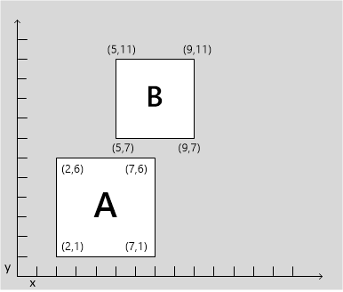
Rectangle	X interval	Y interval
A	{2,7}	{1,6}
B	{5,9}	{7,11}

In pseudocode, that gives us something like:

rectA.IntervalleX.Intersects(rectB.IntervalleX) && rectA.IntervalleY.Intersects(rectB.IntervalleY).

How does interval intersection work? We need four comparisons:

Interval 1 completely contains interval 2: Intervalle1.Min < Intervalle2.Min && Intervalle1.Max > Intervalle2.Max.
Interval 1 is entirely contained within interval 2: Intervalle1.Min > Intervalle2.Min && Intervalle1.Max < Intervalle2.Max.
Interval 1 overlaps the lower end of interval 2: Intervalle1.Min < Intervalle2.Min && Intervalle1.Max > Intervalle2.Min.
Interval 1 overlaps the upper end of interval 2: Intervalle1.min < Intervalle2.Max && Intervalle1.Max > Intervalle2.Max.

Ignoring the possibility of getting a result from the first comparison without running the others, this means at most eight numerical and eight Boolean comparisons: two per comparison, plus one between comparisons. All for a single interval.

Checking two rectangles for intersection therefore requires at most 32 comparisons. That is just two rectangles. With three rectangles, we reach 96, or 32 × 3. Imagine the number of comparisons for all the line segments making up all the roads in France…

This is one of the simplest algorithms for intersecting simple rectangles. Another algorithm uses the rectangles’ centers and radii. Lines, polygons, and other geometric operations have their own algorithms, which are more complex but much more efficient. This example merely illustrates the complexity of these operations and the value of indexing.

Returning to our example, performing every comparison for every road clearly cannot be efficient. A person can also intuitively tell that the Toulouse–Bayonne road will not cross the Nice–Brest railway. Neither will Paris–Strasbourg. Some areas can therefore contain only lines excluded from our result. We need a useful, efficient partitioning scheme that helps exclude geometric objects we already know are irrelevant.

This suggests an interesting solution:

First, run a primary filter that returns a set of possibilities with two properties: it must include every correct result, but may also include objects that do not meet the criteria, or false positives. This filter must be very fast. It can use a division into areas to exclude objects in regions unrelated to our search.
Then run a secondary filter. It is slower, but checks each result precisely, for example by calculating the intersection between the current object and the railway route. It returns exactly the correct results.

This preselection limits the number of records requiring the slow operation without missing any results. That is exactly how SQL Server works.

The geometry and geography types arrived with a new index type: the spatial index. When one exists on a spatial column, it provides the primary filter. It passes a smaller record set to the secondary filter, which, although slow, finishes sooner because it has fewer inputs to analyze. Without an index, the primary filter is bypassed and the secondary filter runs against the entire data set.

Great, but how can that work?

An index needs a sort order to organize the data it references. With int or even varchar, that is straightforward: numerical, alphabetical, or chronological ordering. Geometry and geography types are more complicated because they have no natural order. The answer depends on the data, the space it represents, and its distribution within that space.

You may know that SQL Server organizes indexes as B-trees. These store data in sorted form, allowing insertion and deletion in amortized logarithmic time. In plain language, data is arranged in a particular sorted structure where each node can contain several keys, limiting the rebalancing needed when adding or removing elements.

We therefore need to organize our objects into ranges at several levels. Again, that is easy with numbers — 1–200 containing 1–50, 51–100, 101–150, and 151–200 — but much harder with geometric or geographic shapes.

Index structure

We need a predictable way to divide space while adapting to as many uses as possible. The chosen solution is a grid system. The whole space is divided into a first grid, then each cell is subdivided into another complete grid.

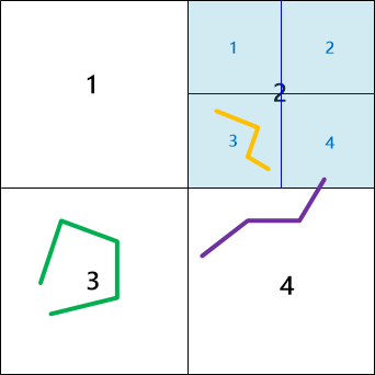
The orange object lies in cell 2 at level 1 and cell 3 at level 2. To answer “Does the green object intersect the orange object?”, reading the first index level is enough.

For the expert

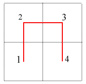
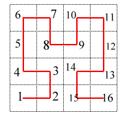
The actual grid-numbering system is much more complex. It uses the Hilbert curve model, a “continuous fractal space-filling curve.” Besides impressing people at parties — although opportunities to mention it are rare :) — this curve can completely fill a space. A one-dimensional curve can fill a two-dimensional space in one continuous stroke. Hilbert curves can also form the basis of mazes. Fun, isn’t it?

Images from http://www.mathcurve.com/fractals/lebesgue/lebesgue.shtml:

A Hilbert curve

A more detailed Hilbert curve

Index distribution

This approach is useful, but if spatial data is spread widely or concentrated into geographic clusters, a 4 × 4 grid may not provide suitable precision. In the following illustration, our data is mostly distributed across five areas. In the northwest, however, the point clouds straddle two level-2 regions.

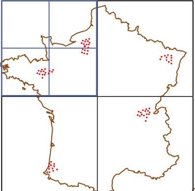
If the query needs level 2, our index is not very selective: it will return at least some points from the other group. Changing the second-level grid to 3 × 3 makes each group fall within a single cell. That is ideal in this example. It will not always hold for your data, but the aim is to optimize as much as possible, and this kind of adjustment can help considerably :).

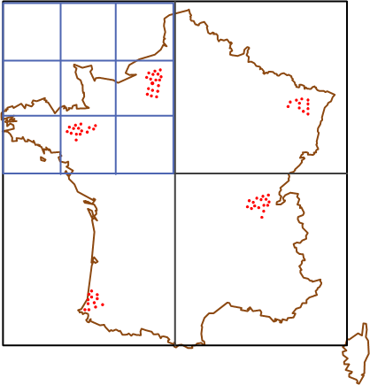
SQL Server’s spatial indexes offer three densities: low, 4 × 4 or 16 cells; medium, 8 × 8 or 64 cells; and high, 16 × 16 or 256 cells. We can therefore increase grid resolution. Higher resolution means a larger index, with greater creation and maintenance costs.

Besides precision, a spatial index has another essential characteristic: four levels. The number is fixed, but each level’s grid density can be adjusted independently; the default is medium. Returning to our road and railway example, we might divide France into 16 cells, then into 64 cells roughly equivalent to half a French department. This configuration could exclude more than half the roads by reading only the first level. Four medium-density levels still represent 64 to the fourth power: 16.7 million cells.

The number matters, but so does distribution. HMMM and MMMH configurations produce the same number of cells, yet their results and performance differ noticeably. Choosing and tuning these settings depends on your data and its distribution.

Building the index

Once the index and its grids are defined, the table’s data must be indexed. SQL Server scans the table row by row. For each object, tessellation places it into the grid hierarchy, starting at the first level and continuing through the four levels if necessary. The resulting set of touched cells is recorded in the spatial index.

This process can be complex, so several rules limit its execution time:

The covering rule: if an object completely covers a cell, that cell is counted as covered and tessellation stops there rather than descending further.
The cells-per-object rule: limits how many cells are counted for one object, except at level 1.
The deepest-cell rule: records only the deepest cells, unless a higher-level cell is entirely covered.

Some of these rules can be adjusted, but that is beyond this article’s scope.

Tessellation has fascinating applications in other areas, including 3D and video games, with developments in DirectX 11. But this post is already long enough Smile . To learn more about tessellation in SQL Server, I recommend TechNet.

Schematic contents of a spatial index

Geometric figure ID	Grid level	Cell number	Covering type
TraitBleu	1,2	2,3	touched
TraitVert	1	3	Partially covered
TraitViolet	1	4	fully covered

Almost everything discussed so far applies to geometry, meaning a plane. Representing the Earth is more complicated. To process information, apply multilevel grids, and calculate distances and intersections, we need a representation of the Earth on a plane: a projection.

The Earth isn’t round!

No, seriously! One of the European Space Agency’s missions illustrates this: GOCE, the Gravity field and steady-state Ocean Circulation Explorer. Look at the geoid, a representation of Earth’s surface based on its gravity field, more precise than other representations.

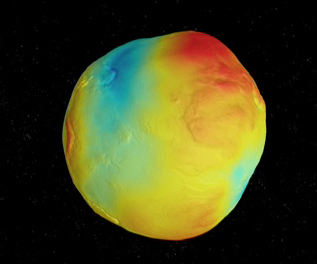
Beyond the anecdote, this may matter considerably in SQL Server. Do your data and calculations use altitude? Do you need precision better than one meter? If so, you probably need to pay attention to the SRID. There are more than 4,000 spatial reference systems, offering different precision globally or over particular parts of the Earth.

Projections are essential for calculations and searches on geographic types. SQL Server performs the projection when needed, based on the objects’ SRID. If projections interest you, read Flat Maps for a Round Planet on MSDN.

Writing queries that use spatial indexes

Your indexes and data are ready: excellent! You can now query in every direction. First, though, make sure the queries you write actually use spatial indexes, at least where performance matters. Only certain methods are supported.

For geography types, only three methods are supported: STIntersects(), STEquals(), and STDistance(). As the documentation explains, these methods must appear in the WHERE clause to use the index.

Geometry types give us more options: STContains(), STDistance(), STEquals(), STIntersects(), STOverlaps(), STTouches(), and STWithin(). Besides WHERE, these methods can appear in JOIN ON clauses.

Note: Filter and STIntersects behave the same without an index. With an index, Filter returns only the equivalent of the primary filter, so false positives are possible.

Spatial index limitations

Spatial indexes can be applied only to geometry or geography columns. You can create at most 249 spatial indexes on a single column in one table. Index creation also cannot take advantage of parallelism on a multicore server.

Their limitations depend heavily on configuration: grid resolution, bounding area, and so on.

The official documentation gives few additional restrictions.

Many geographic operations perform projection. The two hemispheres must be projected separately onto two flat surfaces, making it impossible for a geographic object to span both hemispheres.

Optimizing spatial query performance

sp_help_spatial_geography_index
sp_help_spatial_geometry_index

An article on Todd Jackson’s blog presents an interesting case study. He tested several index configurations against three data sets, ranging from 14,000 to 2.5 million records.

Bounding area and grid resolution

Spatial indexes are always defined on a spatial column over a finite area. For a geography index, the maximum is the entire Earth: longitude −180 to 180 and latitude −90 to 90. It can be reduced, for example if your data covers only France. Geometry data requires a rectangular area. You can also create multiple indexes, one per region, and specify the desired index in a query. That may be useful when each query covers only one region.

As we have seen, grid resolution is also very important and often overlooked. I have no magic recipe for automatically finding the right resolutions for your data and queries, apart from work and careful thought :).

Spatial index hints

Perhaps the first instruction for optimizing spatial queries should be: make sure your index is actually being used! Try forcing it with WITH (INDEX(xsHigh)) at the end of the query and examine the execution plan.

Remember that spatial queries are still queries. You already know how to optimize those ;).